Ludwig Geistlinger
Overview of existing methods for enrichment analysis of gene expression data with regard to functional gene sets, pathways, and networks. Functionality for differential expression analysis, set- and network-based enrichment analysis, along with visualization and exploration of results. Introduction to concepts for enrichment analysis of genomic regions and regulatory elements. Required packages: EnrichmentBrowser, ALL, hgu95av2.db, airway, regioneR, BSgenome.Hsapiens.UCSC.hg19.masked
<img src="https://github.com/waldronlab/BrownCOBRE2018/blob/master/notebooks_day2/ExpressionDataAnalysis.png?raw=true", alt="ExpressionDataAnalysis image", style="width:500px">
Test whether known biological functions or processes are over-represented (= enriched) in an experimentally-derived gene list, e.g. a list of differentially expressed (DE) genes. See Goeman and Buehlmann, 2007 for a critical review.
Example: Transcriptomic study, in which 12,671 genes have been tested for differential expression between two sample conditions and 529 genes were found DE.
Among the DE genes, 28 are annotated to a specific functional gene set, which contains in total 170 genes. This setup corresponds to a 2x2 contingency table,
deTable <-
     matrix(c(28, 142, 501, 12000),
            nrow = 2,
            dimnames = list(c("DE", "Not.DE"),
                            c("In.gene.set", "Not.in.gene.set")))
deTable
where the overlap of 28 genes can be assessed based on the hypergeometric distribution. This corresponds to a one-sided version of Fisher's exact test, yielding here a significant enrichment.
fisher.test(deTable, alternative = "greater")
This basic principle is at the foundation of major public and commercial enrichment tools such as DAVID and Pathway Studio.
Although gene set enrichment methods have been primarily developed and applied on transcriptomic data, they have recently been modified, extended and applied also in other fields of genomic and biomedical research. This includes novel approaches for functional enrichment analysis of proteomic and metabolomic data as well as genomic regions and disease phenotypes, Lavallee and Yates, 2016, Chagoyen et al., 2016, McLean et al., 2010, Ried et al., 2012.
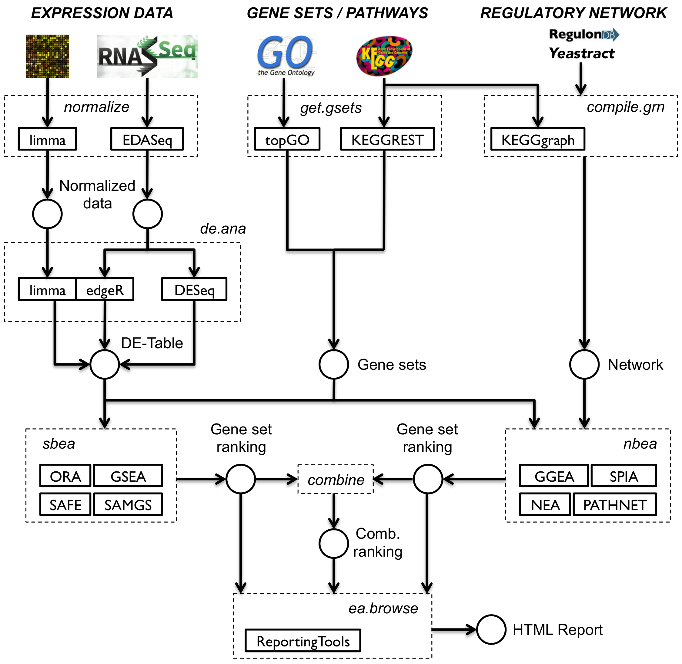
The first part of the workshop is largely based on the EnrichmentBrowser package, which implements an analysis pipeline for high-throughput gene expression data as measured with microarrays and RNA-seq. In a workflow-like manner, the package brings together a selection of established Bioconductor packages for gene expression data analysis. It integrates a wide range of gene set enrichment analysis methods and facilitates combination and exploration of results across methods.
<img src="https://github.com/waldronlab/BrownCOBRE2018/blob/master/notebooks_day2/EnrichmentBrowserWorkflow.png?raw=true", alt="EnrichmentBrowserWorkflow image", style="width:650px">
suppressPackageStartupMessages(library(EnrichmentBrowser))
Further information can be found in the vignette and publication.
Gene sets, pathways & regulatory networks
Gene sets are simple lists of usually functionally related genes without further specification of relationships between genes.
Pathways can be interpreted as specific gene sets, typically representing a group of genes that work together in a biological process. Pathways are commonly divided in metabolic and signaling pathways. Metabolic pathways such as glycolysis represent biochemical substrate conversions by specific enzymes. Signaling pathways such as the MAPK signaling pathway describe signal transduction cascades from receptor proteins to transcription factors, resulting in activation or inhibition of specific target genes.
Gene regulatory networks describe the interplay and effects of regulatory factors (such as transcription factors and microRNAs) on the expression of their target genes.
Resources
GO and KEGG annotations are most frequently used for the enrichment analysis of functional gene sets. Despite an increasing number of gene set and pathway databases, they are typically the first choice due to their long-standing curation and availability for a wide range of species.
GO: The Gene Ontology (GO) consists of three major sub-ontologies that classify gene products according to molecular function (MF), biological process (BP) and cellular component (CC). Each ontology consists of GO terms that define MFs, BPs or CCs to which specific genes are annotated. The terms are organized in a directed acyclic graph, where edges between the terms represent relationships of different types. They relate the terms according to a parent-child scheme, i.e. parent terms denote more general entities, whereas child terms represent more specific entities.
KEGG: The Kyoto Encyclopedia of Genes and Genomes (KEGG) is a collection of manually drawn pathway maps representing molecular interaction and reaction networks. These pathways cover a wide range of biochemical processes that can be divided in 7 broad categories: metabolism, genetic and environmental information processing, cellular processes, organismal systems, human diseases, and drug development. Metabolism and drug development pathways differ from pathways of the other 5 categories by illustrating reactions between chemical compounds. Pathways of the other 5 categories illustrate molecular interactions between genes and gene products.
Gene set analysis vs. gene set enrichment analysis
The two predominantly used enrichment methods are:
However, the term gene set enrichment analysis nowadays subsumes a general strategy implemented by a wide range of methods Huang et al., 2009. Those methods have in common the same goal, although approach and statistical model can vary substantially Goeman and Buehlmann, 2007, Khatri et al., 2012.
To better distinguish from the specific method, some authors use the term gene set analysis to denote the general strategy. However, there is also a specific method from Efron and Tibshirani, 2007 of this name.
Underlying null: competitive vs. self-contained
Goeman and Buehlmann, 2007 classified existing enrichment methods into competitive and self-contained based on the underlying null hypothesis.
Although the authors argue that a self-contained null is closer to the actual question of interest, the vast majority of enrichment methods is competitive.
Goeman and Buehlmann further raise several critical issues concerning the 2x2 ORA:
With regard to these statistical concerns, GSEA is considered superior:
However, the simplicity and general applicability of ORA is unmet by subsequent methods improving on these issues. For instance, GSEA requires the expression data as input, which is not available for gene lists derived from other experiment types. On the other hand, the involved sample permutation procedure has been proven inaccurate and time-consuming Efron and Tibshirani, 2007, Phipson and Smyth, 2010, Larson and Owen, 2015.
Generations: ora, fcs & topology-based
Khatri et al., 2012 have taken a slightly different approach by classifying methods along the timeline of development into three generations:
Although topology-based (also: network-based) methods appear to be most realistic, their straightforward application can be impaired by features that are not-detectable on the transcriptional level (such as protein-protein interactions) and insufficient network knowledge Geistlinger et al., 2013, Bayerlova et al., 2015.
Given the individual benefits and limitations of existing methods, cautious interpretation of results is required to derive valid conclusions. Whereas no single method is best suited for all application scenarios, applying multiple methods can be beneficial. This has been shown to filter out spurious hits of individual methods, thereby reducing the outcome to gene sets accumulating evidence from different methods Geistlinger et al., 2016, Alhamdoosh et al., 2017.
Although RNA-seq (read count data) has become the de facto standard for transcriptomic profiling, it is important to know that many methods for differential expression and gene set enrichment analysis have been originally developed for microarray data (intensity measurements).
However, differences in data distribution assumptions (microarray: quasi-normal, RNA-seq: negative binomial) made adaptations in differential expression analysis and, to some extent, also in gene set enrichment analysis necessary.
Thus, we consider two example datasets - a microarray and a RNA-seq dataset, and discuss similarities and differences of the respective analysis steps.
For microarray data, we consider expression measurements of patients with acute lymphoblastic leukemia Chiaretti et al., 2004. A frequent chromosomal defect found among these patients is a translocation, in which parts of chromosome 9 and 22 swap places. This results in the oncogenic fusion gene BCR/ABL created by positioning the ABL1 gene on chromosome 9 to a part of the BCR gene on chromosome 22.
We load the ALL dataset
library(ALL)
data(ALL)
and select B-cell ALL patients with and without the BCR/ABL fusion, as described previously Gentleman et al., 2005.
ind.bs <- grep("^B", ALL$BT)
ind.mut <- which(ALL$mol.biol %in% c("BCR/ABL", "NEG"))
sset <- intersect(ind.bs, ind.mut)
all.eset <- ALL[, sset]
We can now access the expression values, which are intensity measurements on a log-scale for 12,625 probes (rows) across 79 patients (columns).
dim(all.eset)
exprs(all.eset)[1:4,1:4]
As we often have more than one probe per gene, we compute gene expression values as the average of the corresponding probe values.
all.eset <- probe.2.gene.eset(all.eset)
head(names(all.eset))
For RNA-seq data, we consider transcriptome profiles of four primary human airway smooth muscle cell lines in two conditions: control and treatment with dexamethasone Himes et al., 2014.
We load the airway dataset
library(airway)
data(airway)
For further analysis, we only keep genes that are annotated to an ENSEMBL gene ID.
air.eset <- airway[grep("^ENSG", names(airway)), ]
dim(air.eset)
assay(air.eset)[1:4,1:4]
Normalization of high-throughput expression data is essential to make results
within and between experiments comparable. Microarray (intensity measurements)
and RNA-seq (read counts) data typically show distinct features that need to be
normalized for. As this is beyond the scope of this workshop, we refer to
limma
for microarray normalization and
EDASeq
for RNA-seq normalization. See also EnrichmentBrowser::normalize, which wraps
commonly used functionality for normalization.
The EnrichmentBrowser incorporates established functionality from the
limma
package for differential expression analysis.
This involves the voom transformation when applied to RNA-seq data.
Alternatively, differential expression analysis for RNA-seq data can also be
carried out based on the negative binomial distribution with
edgeR
and
DESeq2.
This can be performed using the function EnrichmentBrowser::de.ana
and assumes some standardized variable names:
For more information on experimental design, see the limma user's guide, chapter 9.
For the ALL dataset, the GROUP variable indicates whether the BCR-ABL gene fusion is present (1) or not (0).
all.eset$GROUP <- ifelse(all.eset$mol.biol == "BCR/ABL", 1, 0)
table(all.eset$GROUP)
For the airway dataset, it indicates whether the cell lines have been treated with dexamethasone (1) or not (0).
air.eset$GROUP <- ifelse(colData(airway)$dex == "trt", 1, 0)
table(air.eset$GROUP)
Paired samples, or in general sample batches/blocks, can be defined via a
BLOCK column in the colData slot. For the airway dataset, the sample blocks
correspond to the four different cell lines.
air.eset$BLOCK <- airway$cell
table(air.eset$BLOCK)
For microarray data, the EnrichmentBrowser::de.ana function carries out
differential expression analysis based on functionality from the
limma package. Resulting log2 fold changes and t-test derived
p-values for each gene are appended to the rowData slot.
all.eset <- de.ana(all.eset)
rowData(all.eset, use.names=TRUE)
Nominal p-values are already corrected for multiple testing (ADJ.PVAL)
using the method from Benjamini and Hochberg implemented in stats::p.adjust.
For RNA-seq data, the de.ana function can be used to carry out differential
expression analysis between the two groups either based on functionality from
limma (that includes the voom transformation), or
alternatively, the frequently used edgeR or DESeq2
package. Here, we use the analysis based on edgeR.
air.eset <- de.ana(air.eset, de.method="edgeR")
rowData(air.eset, use.names=TRUE)
Exercise: Compare the number of differentially expressed genes as obtained on the air.eset with limma/voom, edgeR, and DESeq2.
We are now interested in whether pre-defined sets of genes that are known to
work together, e.g. as defined in the Gene Ontology
or the KEGG pathway annotation, are coordinately
differentially expressed. The function get.kegg.genesets downloads all KEGG
pathways for a chosen organism (here: Homo sapiens) as gene sets using NCBI
Entrez Gene IDs.
kegg.gs <- get.kegg.genesets("hsa")
Analogously, the function get.go.genesets retrieves GO terms of a selected
ontology (here: biological process, BP) as defined in the GO.db
annotation package.
go.gs <- get.go.genesets(org="hsa", onto="BP", mode="GO.db")
User-defined gene sets can be parsed from GMT file format. Here, we are using this functionality for reading a list of already downloaded KEGG gene sets for Homo sapiens containing NCBI Entrez Gene IDs.
data.dir <- system.file("extdata", package="EnrichmentBrowser")
gmt.file <- file.path(data.dir, "hsa_kegg_gs.gmt")
hsa.gs <- parse.genesets.from.GMT(gmt.file)
length(hsa.gs)
hsa.gs[1:2]
See also the MSigDb for additional gene set collections.
A variety of gene set analysis methods have been proposed Khatri et al., 2012. The most basic, yet frequently used, method is the over-representation analysis (ORA) with gene sets defined according to GO or KEGG. As outlined in the first section, ORA tests the overlap between DE genes (typically DE p-value < 0.05) and genes in a gene set based on the hypergeometric distribution. Here, we choose a significance level $\alpha = 0.2$ for demonstration.
ora.all <- sbea(method="ora", eset=all.eset, gs=hsa.gs, perm=0, alpha=0.2)
gs.ranking(ora.all)
Such a ranked list is the standard output of most existing enrichment tools.
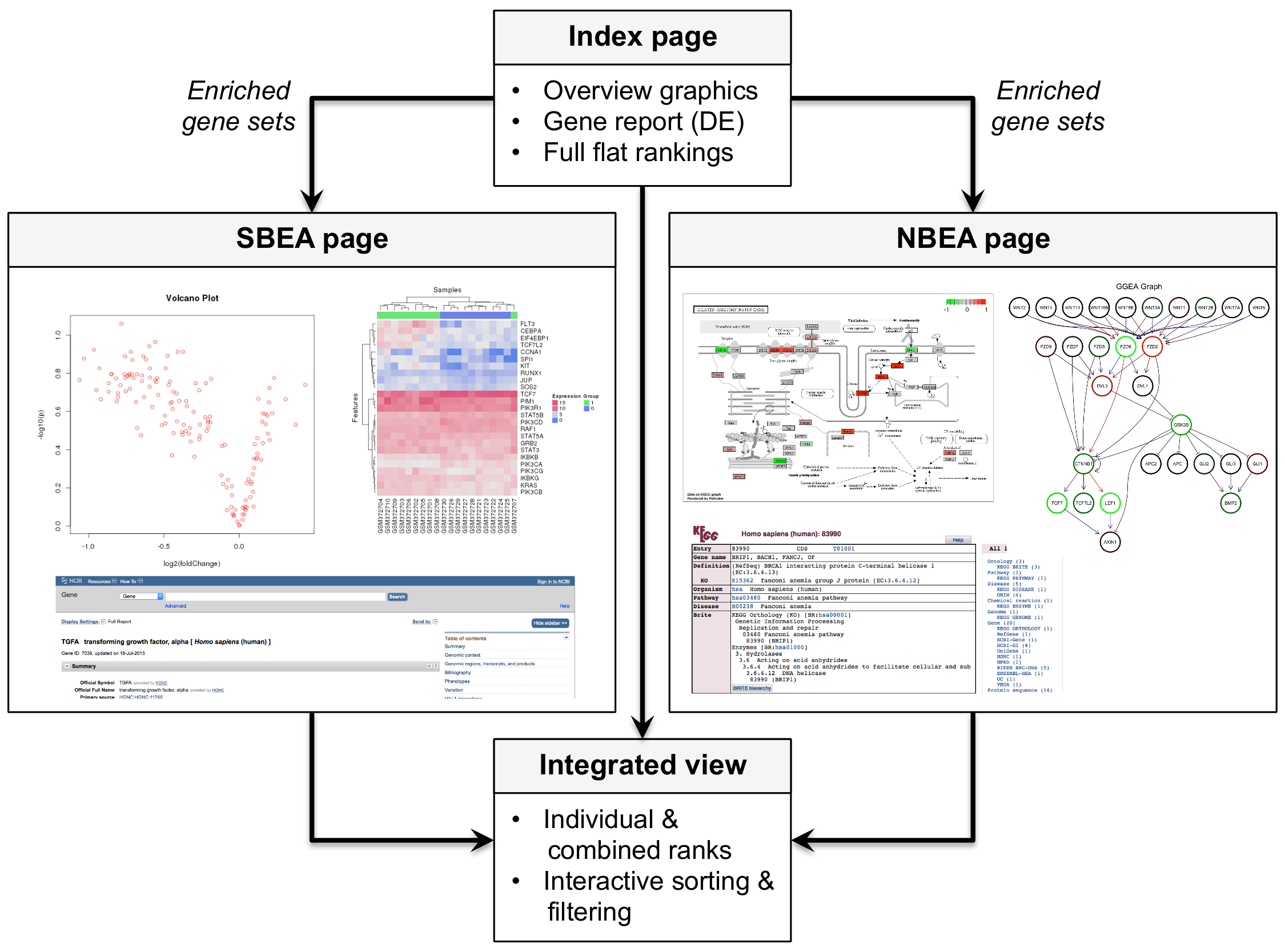
Using the ea.browse function creates a HTML summary from which each
gene set can be inspected in more detail.
<img src="https://github.com/waldronlab/BrownCOBRE2018/blob/master/notebooks_day2/EnrichmentBrowserNavigation.png?raw=true", alt="EnrichmentBrowserNavigation image", style="width:600px">
ea.browse(ora.all)
The resulting summary page includes for each significant gene set
NR.GENES),SET.VIEW, supports mouse-over and click-on),PATH.VIEW, supports mouse-over and click-on).As ORA works on the list of DE genes and not the actual expression values, it can be straightforward applied to RNA-seq data. However, as the gene sets here contain NCBI Entrez gene IDs and the airway dataset contains ENSEMBL gene ids, we first map the airway dataset to Entrez IDs.
air.eset <- map.ids(air.eset, org="hsa", from="ENSEMBL", to="ENTREZID")
ora.air <- sbea(method="ora", eset=air.eset, gs=hsa.gs, perm=0)
gs.ranking(ora.air)
Note #1: Young et al., 2010, have
reported biased results for ORA on RNA-seq data due to over-detection of
differential expression for long and highly expressed transcripts. The
goseq
package and limma::goana implement possibilities to adjust ORA for gene length
and abundance bias.
Note #2: Independent of the expression data type under investigation, overlap between gene sets can result in redundant findings. This is well-documented for GO (parent-child structure, Rhee et al., 2008) and KEGG (pathway overlap/crosstalk, Donato et al., 2013). The topGO package (explicitly designed for GO) and mgsa (applicable to arbitrary gene set definitions) implement modifications of ORA to account for such redundancies.
A major limitation of ORA is that it restricts analysis to DE genes, excluding genes not satisfying the chosen significance threshold (typically the vast majority).
This is resolved by gene set enrichment analysis (GSEA), which scores the tendency of gene set members to appear rather at the top or bottom of the ranked list of all measured genes Subramanian et al., 2005. The statistical significance of the enrichment score (ES) of a gene set is assessed via sample permutation, i.e. (1) sample labels (= group assignment) are shuffled, (2) per-gene DE statistics are recomputed, and (3) the enrichment score is recomputed. Repeating this procedure many times allows to determine the empirical distribution of the enrichment score and to compare the observed enrichment score against it. Here, we carry out GSEA with 1000 permutations.
gsea.all <- sbea(method="gsea", eset=all.eset, gs=hsa.gs, perm=1000)
gs.ranking(gsea.all)
As GSEA's permutation procedure involves re-computation of per-gene DE statistics, adaptations are necessary for RNA-seq. The EnrichmentBrowser implements an accordingly adapted version of GSEA, which allows incorporation of limma/voom, edgeR, or DESeq2 for repeated DE re-computation within GSEA. However, this is computationally intensive (for limma/voom the least, for DESeq2 the most). Note the relatively long running times for only 100 permutations having used edgeR for DE analysis.
gsea.air <- sbea(method="gsea", eset=air.eset, gs=hsa.gs, perm=100)
While it might be in some cases necessary to apply permutation-based GSEA for RNA-seq data, there are also alternatives avoiding permutation. Among them is ROtAtion gene Set Testing (ROAST), which uses rotation instead of permutation Wu et al., 2010.
roast.air <- sbea(method="roast", eset=air.eset, gs=hsa.gs)
gs.ranking(roast.air)
A selection of additional methods is also available:
sbea.methods()
Exercise: Carry out a GO overrepresentation analysis for the all.eset and air.eset. How many significant gene sets do you observe in each case?
Having found gene sets that show enrichment for differential expression, we are now interested whether these findings can be supported by known regulatory interactions.
For example, we want to know whether transcription factors and their target genes are expressed in accordance to the connecting regulations (activation/inhibition). Such information is usually given in a gene regulatory network derived from specific experiments or compiled from the literature (Geistlinger et al., 2013 for an example).
There are well-studied processes and organisms for which comprehensive and well-annotated regulatory networks are available, e.g. the RegulonDB for E. coli and Yeastract for S. cerevisiae.
However, there are also cases where such a network is missing or at least incomplete. A basic workaround is to compile a network from regulations in the KEGG database.
We can download all KEGG pathways of a specified organism (here: Homo sapiens) via
But for demonstration purposes, we use a selection of already downloaded human KEGG pathways:
pwys <- file.path(data.dir, "hsa_kegg_pwys.zip")
hsa.grn <- compile.grn.from.kegg(pwys)
head(hsa.grn)
Signaling pathway impact analysis (SPIA) is a network-based enrichment analysis method, which is explicitly designed for KEGG signaling pathways Tarca et al., 2009. The method evaluates whether expression changes are propagated across the pathway topology in combination with ORA.
spia.all <- nbea(method="spia", eset=all.eset, gs=hsa.gs, grn=hsa.grn, alpha=0.2)
gs.ranking(spia.all)
More generally applicable is gene graph enrichment analysis (GGEA), which evaluates consistency of interactions in a given gene regulatory network with the observed expression data Geistlinger et al., 2011.
ggea.all <- nbea(method="ggea", eset=all.eset, gs=hsa.gs, grn=hsa.grn)
gs.ranking(ggea.all)
A selection of additional network-based methods is also available:
nbea.methods()
Note #1: As network-based enrichment methods typically do not involve sample permutation but rather network permutation, thus avoiding DE re-computation, they can likewise be applied to RNA-seq data.
Note #2: Given the various enrichment methods with individual benefits and limitations, combining multiple methods can be beneficial, e.g. combined application of a set-based and a network-based method. This has been shown to filter out spurious hits of individual methods and to reduce the outcome to gene sets accumulating evidence from different methods Geistlinger et al., 2016, Alhamdoosh et al., 2017.
The function comb.ea.results implements the straightforward combination of
results, thereby facilitating seamless comparison of results across methods.
For demonstration, we use the ORA and GSEA results for the ALL dataset from the
previous section:
res.list <- list(ora.all, gsea.all)
comb.res <- comb.ea.results(res.list)
gs.ranking(comb.res)
Exercise: Carry out SPIA and GGEA for the air.eset and combine the results. How many gene sets are rendered significant by both methods?
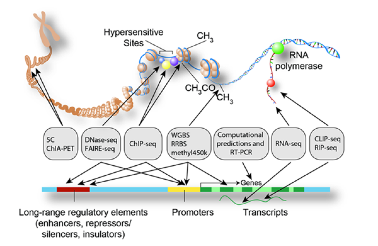
Microarrays and next-generation sequencing are also widely applied for large-scale detection of variable and regulatory genomic regions, e.g. single nucleotide polymorphisms, copy number variations, and transcription factor binding sites.
<img src="https://github.com/waldronlab/BrownCOBRE2018/blob/master/notebooks_day2/ENCODE.png?raw=true", alt="ENCODE image", style="width:600px">
Such experimentally-derived genomic region sets are raising similar questions regarding functional enrichment as in gene expression data analysis.
Of particular interest is thereby whether experimentally-derived regions overlap more (enrichment) or less (depletion) than expected by chance with regions representing known functional features such as genes or promoters.
The regioneR package implements a general framework for testing overlaps of genomic regions based on permutation sampling. This allows to repeatedly sample random regions from the genome, matching size and chromosomal distribution of the region set under study. By recomputing the overlap with the functional features in each permutation, statistical significance of the observed overlap can be assessed.
suppressPackageStartupMessages(library(regioneR))
To demonstrate the basic functionality of the package, we consider the overlap of gene promoter regions and CpG islands in the human genome. We expect to find an enrichment as promoter regions are known to be GC-rich. Hence, is the overlap between CpG islands and promoters greater than expected by chance?
We use the collection of CpG islands described in Wu et al., 2010 and restrict them to the set of canonical chromosomes 1-23, X, and Y.
cpgHMM <- toGRanges("http://www.haowulab.org/software/makeCGI/model-based-cpg-islands-hg19.txt")
cpgHMM <- filterChromosomes(cpgHMM, chr.type="canonical")
cpgHMM <- sort(cpgHMM)
cpgHMM
Analogously, we load promoter regions in the hg19 human genome assembly as available from UCSC:
promoters <- toGRanges("http://gattaca.imppc.org/regioner/data/UCSC.promoters.hg19.bed")
promoters <- filterChromosomes(promoters, chr.type="canonical")
promoters <- sort(promoters)
promoters
To speed up the example, we restrict analysis to chromosomes 21 and 22. Note that this is done for demonstration only. To make an accurate claim, the complete region set should be used (which, however, runs considerably longer).
cpg <- cpgHMM[seqnames(cpgHMM) %in% c("chr21", "chr22")]
prom <- promoters[seqnames(promoters) %in% c("chr21", "chr22")]
Now, we are applying an overlap permutation test with 100 permutations
(ntimes=100), while maintaining chromosomal distribution of the CpG island
region set (per.chromosome=TRUE). Furthermore, we use the option
count.once=TRUE to count an overlapping CpG island only once, even if it
overlaps with 2 or more promoters.
This takes about 2 minutes on a standard laptop. It also takes too much memory for the machines used by the workshop, so the command is commented out and the object loaded from file instead.
# pt <- overlapPermTest(cpg, prom, genome="hg19", ntimes=100, per.chromosome=TRUE, count.once=TRUE)
download.file("https://www.dropbox.com/s/dlqq0m99wpu5xab/BrownCOBREDay2Session3_pt.rds?raw=1", destfile="BrownCOBREDay2Session3_pt.rds")
pt <- readRDS("BrownCOBREDay2Session3_pt.rds")
pt
summary(pt[[1]]$permuted)
The resulting permutation p-value indicates a significant enrichment. Out of the 2859 CpG islands, 719 overlap with at least one promoter. In contrast, when repeatedly drawing random regions matching the CpG islands in size and chromosomal distribution, the mean number of overlapping regions across permutations was 117.7 $\pm$ 11.8.
Note #1: The function regioneR::permTest allows to incorporate user-defined
functions for randomizing regions and evaluating additional measures of overlap
such as total genomic size in bp.
Note #2: The LOLA package implements a genomic region ORA, which assesses genomic region overlap based on the hypergeometric distribution using a library of pre-defined functional region sets.