Brown Univ. Introduction to Bioconductor 2018, Period 2
Genomic ranges for organizing and interrogating genome-scale data
Period 2 has the following basic outline. We want to understand the basic IRanges and GRanges infrastructure components and then use them to organize and interrogate genomic experiments.
Period II. Working with general genomic features using GenomicRanges
  IRanges introduced
  Intra-range operations
  Inter-range operations
  GRanges
  Calculating overlaps
Range-oriented solutions for current experimental paradigms
  GenomicFiles for families of BAM or BED
SummarizedExperiment: for RNA-seqsuppressPackageStartupMessages({ # basic setup tasks
library(IRanges)
library(Homo.sapiens)
library(GenomicRanges)
library(gwascat)
library(BiocStyle)
library(RNAseqData.HNRNPC.bam.chr14)
library(GenomicFiles)
library(erma)
library(rtracklayer)
})
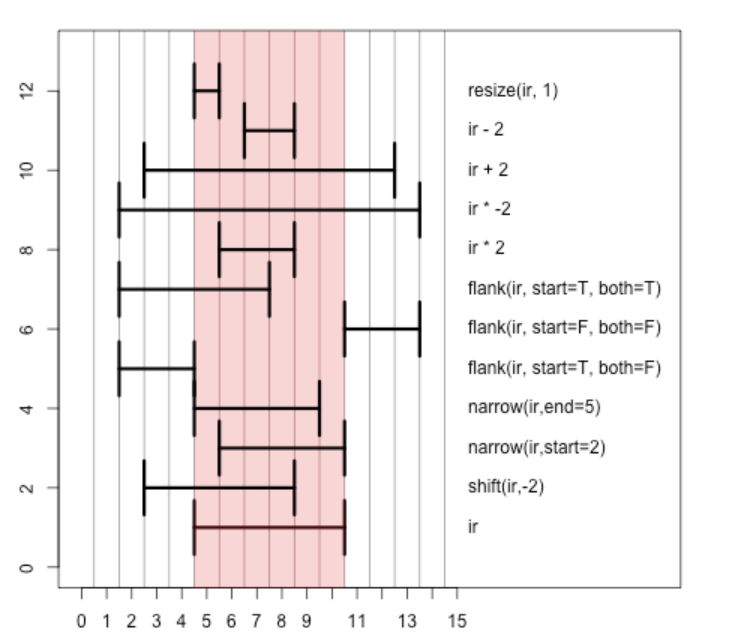
Intra-range operations
We are working with the positions in the interval [5, 10], shaded pink above. We will learn how to interpret the methods
shift, narrow, flank, resize, and various arithmetic operations.
We create our basic IRanges instance:
ir = IRanges(5, 10)
ir
Now function calls for selected 'intra-range' operations.
shift(ir, -2)
resize(ir, 1)
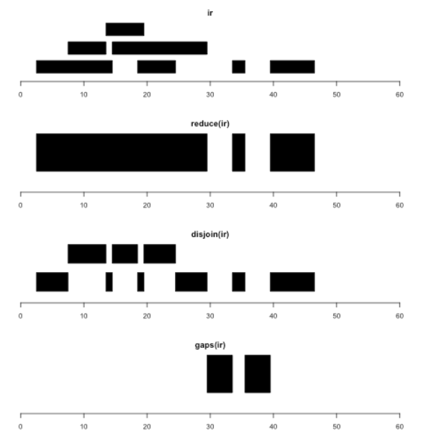
Multi-range objects
We can create a family of ranges using vector inputs to the IRanges method.
ir <- IRanges(c(3, 8, 14, 15, 19, 34, 40),
  width = c(12, 6, 6, 15, 6, 2, 7))
ir
This range set is displayed in the figure below. The intra-range operations will be applied elementwise.
resize(ir,1) # leftmost width-1 position
Inter-range operations
Information about inter-range operations can be obtained using ?"inter-range-methods". For example, for a multi-range instance ir, reduce(ir)
produces a new IRanges instance representing the merging of all locations occupied by any range.
reduce(ir)
Metadata and indexing for ranges
We can give names to ranges, associate multiple fields of metadata to each range (using mcols), and use bracket-style indexing.
names(ir) = letters[1:7]
ir[c("a", "d")]
The association of a collection of attributes with each range is very useful for genomic annotation. Any
conformant data.frame instance (one row per range) can be used with the mcols assignment operation to
annotate a set of ranges. We use some attributes of the mtcars dataset for illustration.
mcols(ir) = mtcars[1:7,1:3]
ir
resize(ir,1) # metadata are propagated for intra-range operations
gaps(ir) # not for inter-range operations
IRanges is the name of a formal class, and we can enumerate all known methods on this class:
length(methods(class="IRanges"))
Clearly there is substantial infrastructure defined for this concept. The roles of some of these methods in genome-scale analysis becomes clearer in the next section.
Exercises
The ir object that combines ranges with some information on car models is completely contrived
but the following questions should be manageable.
Write the code to determine the maximum width of ranges corresponding to 6 cylinder cars.
max(width(ir[mcols(ir)$cyl==6]))
Show that the average value of miles per gallon for cars corresponding to ranges with start values greater than 14 is 18.125.
Finding overlapping regions
The problem of finding overlaps among collections of intervals is commonly encountered. There are
various nuances covered in the documentation. We'll use our collection of intervals ir to
illustrate the basic idea. We'll break the set into two groups.
ir1 = ir[c(3,7)]
ir2 = ir[-c(3,7)]
ir1
ir2
We then use findOverlaps, which has two obligatory arguments: query, and subject.
fo = findOverlaps(ir1, ir2) # ir1 is query, ir2 is subject
fo
The elements of ir2 that were overlapped by ranges in ir1 are listed as follows:
ir2[subjectHits(fo)]
A logical vector indicating which elements of ir1 overlapped elements of ir2 can be computed as
ir1 %over% ir2
GRanges to handle the context of genomic coordinates
Base positions and intervals on genomic sequences can be modeled using IRanges, but it is essential
to add metadata that establish a number of contextual details. It is typical to maintain information
about chromosome identity and chromosome length, along with labels for genome build and origin.
We saw one example early on: apply the genes method to Homo.sapiens.
library(Homo.sapiens)
hg = genes(Homo.sapiens)
hg
There is an obligatory metadata construct called seqnames that gives the chromosome occupied by the gene whose start and end positions are modeled by the associated IRanges. Strand is also recorded.
Plus strand features have the biological direction from left to right on the number line, and minus strand features have the biological direction from right to left. In terms of the IRanges, plus strand features go from start to end, and minus strand features go from end to start. This is required because width is defined as end - start + 1, and negative width ranges are not allowed. Because DNA has two strands, which have an opposite directionality, strand is necessary for uniquely referring to DNA.
Strand may have values +, -, or * for unspecified. seqinfo collects information on the chromosome names, lengths, circularity, and reference build.
Mildly advanced exercise
You might find the ordering of ranges shown above unpleasant. We can order them by chromosome:
hg[order(seqnames(hg))]
Add code that orders the ranges by starting position within chromosome.
Vector operations
GRanges can be treated as any standard vector.
hg[1:4] # first four in the lexical ordering of `names(hg)`
sort(hg)[1:4] # physical ordering on plus strand
savestrand = strand(hg)
strand(hg) = "*"
sort(hg)[1:4] # different!
strand(hg) = savestrand # restore
Multichromosome context
seqinfo is an important method for/component of well-annotated GenomicRanges instances.
seqinfo(hg)
sum(isCircular(hg), na.rm=TRUE) # how many circular chromosomes?
seqinfo(hg)["chrM"]
# table(seqnames(hg)) # counts of genes per chromosome (or random/unmapped contig)
hg[ which(seqnames(hg)=="chr22") ]
hgs = keepStandardChromosomes(hg, pruning.mode="coarse") # eliminate random/unmapped
hgs
table(seqnames(hgs))
GRangesList for grouped genomic elements
Exons are elements of gene models. The exons method gives a flat sequence of GRanges recording exon positions. exonsBy organizes the exons into genes, yielding a special structure called GRangesList.
ebg = exonsBy(Homo.sapiens, by = "gene")
ebg
Exercise
Note that the unlist(ebg) is efficiently computed and retains the gene entrez id as the name of each exon range. Give the entrez id of the gene with the longest exon.
# keepStandardChromosomes(ebg, pruning.mode="coarse")
Strand-aware operations
Here we present code that helps visualize strand-awareness of GRanges operations. We will
assign strands for the ranges used above and then plot the results of operations that could represent
isolation of transcription-start sites (resize(...,1)), identifying upstream promoter regions
(flank(...,[len])) or downstream promoter regions (flank, ..., len, start=FALSE).
plotGRanges = function (x, xlim = x, col = "black", sep = 0.5, xlimits = c(0,
    60), ...)
{
    main = deparse(substitute(x))
    ch = as.character(seqnames(x)[1])
    x = ranges(x)
    height <- 1
    if (is(xlim, "Ranges"))
        xlim <- c(min(start(xlim)), max(end(xlim)))
    bins <- disjointBins(IRanges(start(x), end(x) + 1))
    plot.new()
    plot.window(xlim = xlimits, c(0, max(bins) * (height + sep)))
    ybottom <- bins * (sep + height) - height
    rect(start(x) - 0.5, ybottom, end(x) + 0.5, ybottom + height,
        col = col, ...)
    title(main, xlab = ch)
    axis(1)
}
Now we can set up the GRanges and strand information to visualize the various elements.
par(mfrow=c(4,1), mar=c(4,2,2,2))
library(GenomicRanges)
gir = GRanges(seqnames="chr1", ir, strand=c(rep("+", 4), rep("-",3)))
plotGRanges(gir, xlim=c(0,60))
plotGRanges(resize(gir,1), xlim=c(0,60),col="green")
plotGRanges(flank(gir,3), xlim=c(0,60), col="purple")
plotGRanges(flank(gir,2,start=FALSE), xlim=c(0,60), col="brown")

An application of findOverlaps with the GWAS catalog
Genome-wide association studies (GWAS) are systematically catalogued in a resource managed at EMBL/EBI. We can retrieve a version of the catalog using the gwascat package.
library(gwascat)
data(ebicat37)
ebicat37
There is one range per GWAS finding. Each range corresponds to a SNP for which an association with a given phenotype is statistically significant, and is replicated. The mcols record many types of data describing the study and the SNP.
Notice that the genome is labelled "GRCh37". This is very similar to hg19. We'll simply alter the tag. If we did not, we would encounter an 'incompatible genomes error'.
genome(ebicat37) = "hg19"
Now we will use findOverlaps to determine which genes have annotated intervals (we'll unpack this concept later) that overlap GWAS hits.
goh = findOverlaps(hg, ebicat37)
goh
We obtain an instance of the Hits class, which records the indices of query ranges and subject ranges that satisfy the default overlap condition.
length(unique(queryHits(goh)))
We have counted the number of genes that overlap one or more GWAS hits. To determine the proportion of SNPs with GWAS associations that lie within gene regions:
mean(reduce(ebicat37) %over% hg)
The same pattern can be used to estimate the proportion of SNP that are GWAS hits lying in exons:
mean(reduce(ebicat37) %over% exons(Homo.sapiens))
Using our crude concept of promoter region (uniform in size for each gene, see ?promoters after attaching GenomicRanges), we can estimate the proportion of SNP that are GWAS hits lying in promoters.
pr = suppressWarnings(promoters(hg, upstream=20000)) # will slip over edge of some chromosomes
pr = keepStandardChromosomes(pr, pruning.mode="coarse")
mean(reduce(ebicat37) %over% pr)
You can use other Bioconductor annotation resources to obtain a more refined definition of 'promoter'.
Working with GRanges and assay collections
A collection of bed files
The erma package was created to demonstrate the use of the GenomicFiles discipline for interactive computing with collections of BED files. (erma abbreviates Epigenomic RoadMap Adventures.) The data have been selected from the roadmap portal, specifically this folder.
These BED files have tabix-indexed. This allows accelerated retrieval of data lying in specified genomic intervals.
We begin by attaching the package and creating an ErmaSet instance.
library(erma)
erset = makeErmaSet()
erset
The colData method extracts information concerning the different files. In this case, each
file corresponds to the classification of genomic intervals in a given cell type according to
the chromatin state labeling algorithm 'ChromHmm'.
In the following cell, we will use a nice method of rendering large tables when using HTML. The DT package includes bindings to javascript functions that render searchable tables.
library(DT)
datatable(as.data.frame(colData(erset)))
colData is analogous to the pData that we saw in dealing with the ExpressionSet class.
The $ shortcut is available.
table(erset$ANATOMY)
The purpose of this collection is to illustrate how we might work with cell-type-specific information on
chromatin state to interpret other genome-scale findings. A key Bioconductor package for working with
BED files is rtacklayer. We'll use the import
method to extract information from one interval in one file.
library(rtracklayer)
import(files(erset)[1], which=GRanges("chr1", IRanges(1e6,1.1e6)))
The next file in the collection gives a different collection of chromatin state labels for a different cell type.
import(files(erset)[2], which=GRanges("chr1", IRanges(1e6,1.1e6)))
The stateProfile function uses extractions of this sort to illustrate the layout of chromatin states
in intervals upstream of gene coding regions.
stateProfile(erset[,26:31], symbol="IL33", upstream=1000, shortCellType=FALSE)

Detailed information about the different states is provided in the erma vignette.
In summary
- BED files are commonly encountered representations of outputs of genome-scale experiments
- Collections of BED files can be managed with GenomicFiles objects
- file-level data are bound in as
colData - intervals of interest are bound in using
rowRanges
- file-level data are bound in as
- We use rtracklayer::import to retrieve detailed information from BED files
- An approach to high-level visualization of chromatin states across diverse cell types is provided in erma::stateProfile
Exercise
There are 15 samples with anatomy label 'BLOOD'. List their cell types, using the Standardized.Epigenome.name
component of the colData(erset).
#data.frame(celltype=colData(erset[...
A collection of BAM files
The package RNAseqData.HNRNPC.bam.chr14 includes BAM representation of reads derived from an experiment studying the effect of knocking down HNRNPC (the gene coding for heterogeneous nuclear ribonucleoproteins C1/C2) in HeLa cells. The purpose of the experiment is to test the hypothesis that these ribonucleoproteins have a role in preventing erroneous inclusion of Alu elements in transcripts. HNRNPC is located on chr14, and the package has filtered reads from 8 runs to those aligning on chr14.
Setting up the GenomicFiles container
We will use a class and a method from the GenomicFiles package to manage and query the BAM files. The locations of the files are present in the vector RNAseqData.HNRNPC.bam.chr14_BAMFILES.
library(RNAseqData.HNRNPC.bam.chr14)
library(GenomicFiles)
gf = GenomicFiles(files=RNAseqData.HNRNPC.bam.chr14_BAMFILES)
gf
Defining a region of interest
Note that the object gf is self-describing and has 0 ranges. We bind a GRanges to this object to
define focus for upcoming operations. The GRanges that we use corresponds to the location of HNRNPC.
rowRanges(gf) = GRanges("chr14", IRanges(21677295,21737638))
gf
Adding sample-level data
We can also assign colData to define aspects of the samples.
colData(gf) = DataFrame(trt=rep(c("WT", "KO"), c(4,4)))
gf$trt
A simple method of counting reads aligning to an interval
In the next section we will apply a black-box function that we will study more carefully latter. We are using summarizeOverlaps in GenomicAlignments. The purpose is to tabulate the counts of reads aligned to HNRNPC.
library(BiocParallel)
register(SerialParam())  # can be altered for multicore machines or clusters
hc = suppressWarnings(summarizeOverlaps(rowRanges(gf), files(gf), singleEnd=FALSE)) # some ambiguous pairing
hc
summarizeOverlaps returns a new type of object that we will examine more closely below. For the
moment, we are concerned with retrieving the read counts from this object, and this uses the assay method.
assay(hc)
These are raw counts. We will talk about normalization and statistical inference later in the course.
SummarizedExperiment for mature assay collections
The SummarizedExperiment class is defined in the SummarizedExperiment package. We implicitly created one with
summarizeOverlaps just above. That was peculiar because it involved only one gene. The general
situation is schematized here:
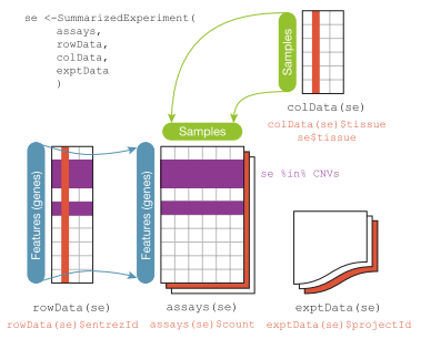
There are "tables" devoted to the features (rowData or rowRanges), assay outputs (assays), and samples (colData).
We'll get acquainted with a typical RNA-seq experiment using the airway package.
library(airway)
data(airway)
airway
Subsets of the SummarizedExperiment are obtained using the X[G, S] idiom. Here we confine attention to 6 features on five samples and extract the counts.
assay(airway[1:6,1:5])
Metadata about the features is recorded at the exon level, in a GRangesList instance. Full details about how the counts were derived is in the vignette for the airway package, and additional approaches are described in Mike Love's notes.
rowRanges(airway)
The sample level data is obtained using colData:
colData(airway)
Exercise
Here is a variation on the twoSamplePlot function that works for SummarizedExperiments. We skip the handling of gene symbols. Given that ENSG00000103196 is the identifier for CRISPLD2, create the visualization comparing expression of this gene in dexamethasone treated samples to controls.
twoSamplePlotSE = function(se, stratvar, rowname) {
    boxplot(split(assay(se[rowname,]),
                  se[[stratvar]]),xlab=stratvar, ylab=rowname)
}
Comment
The two plotting functions differ because of the different methods required to extract assay results. One way to unify them is to branch within the data preparation step.
makeframe = function(x, rowind, colvar) {
     if (is(x, "ExpressionSet")) xv = exprs
         else if (is(x, "SummarizedExperiment")) xv = assay
     ans = data.frame(t(xv(x[rowind,])), p=x[[colvar]], check.names=FALSE)
     names(ans)[2] = colvar
     ans
     }
makeframe(airway, "ENSG00000103196", "dex")
There is still the matter of our ability to take advantage of the gene-symbol resolution that we had for the ExpressionSet with fData component. Achieving semantic uniformity across different data representations is a considerable way off. Sometimes you will have to do lookups with reference data objects, sometimes you can look 'within' the data object to get the desired notation mapping.
Wrapping up
- IRanges represent intervals
- GRanges use IRanges to represent genomic regions
- seqnames typically identifies chromosome
- mcols can be used to annotate regions
- intra-range and inter-range operations are implemented efficiently
- the locations of all human genes is given by genes(Homo.sapiens)
- the GWAS catalog can be represented as a GRanges
- findOverlaps can be used to identify common locations for diverse phenomena
- GenomicFiles manages collections of BED or similar files
- file-level (or sample-level) metadata are bound in with colData
- regions of interest are bound in with rowRanges
- rtracklayer::import extracts quantitative information and metadata
- erma::stateProfile illustrates cell-type-specific variation in chromatin states near genes of interest
- GenomicFiles can manage BAM collections (see also BamFileList)
- summarizeOverlaps can obtain read counts in regions of interest
- SummarizedExperiment coordinates information on samples, features, and assay outputs for many types of experiments