Brown Univ. Introduction to Bioconductor 2018, Period 1
A comment on how to use the notebook
It is probably best to "clear" all cells at first. We will go through text, look at the code blocks, think about what they mean, and then execute them. Use the "Cell" tab and select "All Output", then click on the "Clear" option that will appear.
Road map
- Overview of Bioconductor project and statement of some core values
- Installation and documentation briefly reviewed
- Coordinating information from multiple files in ExpressionSets
- Using GEOquery to obtain annotated expression data from NCBI GEO
Specifically we will work with data from a Cancer Cell paper that "show[s] that LXR-623, a clinically viable, highly brain-penetrant LXRα-partial/LXRβ-full agonist selectively kills GBM cells in an LXRβ- and cholesterol-dependent fashion, causing tumor regression and prolonged survival in mouse models."
Motivations and core values
# a quick setup to avoid extraneous messages
suppressPackageStartupMessages({
    library(Homo.sapiens)
    library(GEOquery)
    library(GSE5859Subset)
    library(Biobase)
    library(pasilla) # or make sure it is installed
})
Why R?
Bioconductor is based on R. Three key reasons for this are:
R is used by many statisticians and biostatisticians to create algorithms that advance our ability to understand complex experimental data.
R is highly interoperable, and fosters reuse of software components written in other languages.
R is portable to the key operating systems running on commodity computing equipment (Linux, MacOSX, Windows) and can be used immediately by beginners with access to any of these platforms.
Other languages are starting to share these features. However the large software ecosystems of R and Bioconductor will continue to play a role even as new languages and environments for genome-scale analysis start to take shape.
What is R?
We'll see more clearly what R is as we work with it. Two features that merit attention are its approach to functional and object-oriented programming.
Before we get into these programming concepts, let's get clear on the approach we are taking to working with R.
- We are using R interactively in the Jupyter notebook system for scientific computing
- Our interaction with R is defined in notebook "cells"
- We can put some code in a cell and ask the notebook server to execute the code
- If there's an error or we want to modify the cell for some reason, we just change the content of the cell and request a new execution
Defining and using functions
The next two cells introduce a simple R function and then pose some questions that you can answer by modifying the second cell.
# functional programming example
cube = function(x) x^3
cube(4)
Exercises
Ex1. What is the cube of 7? Use the cube function
cube(7)
Ex2. Given the cube function, what is a concise way of defining a function that computes the ninth power of its argument, without invoking the exponential directly?
nin = function(x) cube(cube(x))
    nin(4)
    4^9
To review:
g = function(x, y, ...) { --- }is R syntax to define a new function named "g" accepting a series of arguments.- The body of the function (denoted
{ --- }) uses the inputs and R programming to compute new values. - All program actions in R result from evaluating functions.
What is Bioconductor?
While Bioconductor is built on R, a number of distinctions are worthy of attention:
| R | Bioconductor |
|---|---|
| a general-purpose programming for statistical computing and visualization | R data structures, methods, and packages for Bioinformatics |
| a decentralized open-source project | led by a Core Team of full-time developers |
provides methods primarily acting on generic data structures like numeric, matrix, data.frame, and "tidyverse" alternatives like tibble |
provides methods primarily acting on integrative data structures for -omics like GRanges and SummarizedExperiment |
| is enhanced by the CRAN,ecosystem of >10K add-packages spanning all areas of science,,economics, computing, etc | an ecosystem of >1,200 add-on packages |
| CRAN enforces basic package requirements of man pages,and clean machine checks | Bioconductor enforces additional package requirements of vignettes, re-use of core Bioconductor data structures, unit tests |
| Wikipedia describes aspects of commercially supported versions of R | Bioconductor development is supported by several NIH and EC grants |
Working with objects
Genome-scale experiments and annotations are complex. The discipline of object-oriented programming became popular in the 1990s as a way of managing program complexity. Briefly, we think of a class of objects -- say 'organism'. Methods that apply to directly to instances of the 'organism' class include 'genes', 'transcripts', 'promoters'.
This concept is implemented fairly directly in Bioconductor, but there are gaps in certain places. Let's
just explore to establish a little familiarity. We'll attach the Homo.sapiens library, which gives us access to an
object called Homo.sapiens, which answers to a certain collection of methods.
library(Homo.sapiens)
methods(class=class(Homo.sapiens))
genes(Homo.sapiens) # we'll look at this data structure in great detail later
One benefit of the object-oriented discipline is that the same methods apply for different species -- once you have learned how to work with Homo.sapiens, the same tools apply for Mus.musculus, Rattus.norvegicus and so on.
Upshots
We've seen three important facets of the language/ecosystem
- improvised software creation through user-defined functions
- high-level concepts can be expressed as methods applicable to objects (instances of formally defined classes)
- acquisition of complex, biologically meaningful 'objects' and 'methods' with library()
Use of library() is essential to acquire access to functions and documentation on library components. This can be a stumbling block if you remember the name of a function of interest, but not the package in which it is defined.
Another feature worth bearing in mind: all computations in R proceed by evaluation of functions. You may write scripts, but they will be sequences of function calls. One prominent developer (D. Eddelbuettel) has written that "Anything you do more than three times should be a function, and every function should be in a package". Thus full appreciation of R's potentials in scientific computing will ultimately involve understanding of function design and package creation and maintenance.
Thus there are many ways of using software in R.
- write scripts and execute them at a command line using Rscript or unix-like pipes.
- use a bespoke interactive development environment like Rstudio
- use R as a command-line interpreter
- use jupyter notebooks
- use R through online "apps", often composed using the shiny package.
We'll explore some of these alternate approaches as we proceed.
Putting it all together
Bioconductor’s core developer group works hard to develop data structures that allow users to work conveniently with genomes and genome-scale data. Structures are devised to support the main phases of experimentation in genome scale biology:
- Parse large-scale assay data as produced by microarray or sequencer flow-cell scanners.
- Preprocess the (relatively) raw data to support reliable statistical interpretation.
- Combine assay quantifications with sample-level data to test hypotheses about relationships between molecular processes and organism-level characteristics such as growth, disease state.
- In this course we will review the objects and functions that you can use to perform these and related tasks in your own research.
Bioconductor installation and documentation
Installation support
Once you have R you can obtain a utility for adding Bioconductor packages with
source("http://www.bioconductor.org/biocLite.R")This is sensitive to the version of R that you are using. It installs and loads the BiocInstaller package. Let's illustrate its use.
library(BiocInstaller)
biocLite("genomicsclass/GSE5859Subset", suppressUpdates=TRUE, suppressAutoUpdate=TRUE)  # this will be used later
Documentation
For novices, large-scale help resources are always important.
- Bioconductor's main portal has sections devoted to installation, learning, using, and developing. There is a twitter feed for those who need to keep close by.
- The support site is active and friendly
- R has extensive help resources at CRAN and within any instance
# help.start() -- may not work with notebooks but very useful in Rstudio or at command line
Documentation on any base or Bioconductor function can be found using the ?-operator
?mean # use ?? to find documentation on functions in all installed packages
All good manual pages include executable examples
example(lm)

We can get 'package level' help -- a concise description and list of documented functions.
help(package="genefilter", help_type="html") # generates embedded view of DESCRIPTION and function index
Large-scale documentation that narrates and illustrates package (as opposed to function) capabilities is provided in vignettes.
# vignette() # This will generate an HTML page in notebook
# vignette("create_objects", package="pasilla") # this will start the browser to a vignette document
In summary: documentation for Bioconductor and R utilities is diverse but discovery is supported in many ways. RTFM.
Data structure and management for genome-scale experiments
Data management is often regarded as a specialized and tedious dimension of scientific research.
- Because failures of data management are extremely costly in terms of resources and reputation, highly reliable and efficient methods are essential.
- Customary lab science practice of maintaining data in spreadsheets is regarded as risky. We want to add value to data by making it easier to follow reliable data management practices.
In Bioconductor, principles that guide software development are applied in data management strategy.
- High value accrues to data structures that are modular and extensible.
- Packaging and version control protocols apply to data class definitions.
- We will motivate and illustrate these ideas by
- giving examples of transforming spreadsheets to semantically rich objects,
- working with the NCBI GEO archive,
- dealing with families of BAM and BED files, and (optionally)
- using external storage to foster coherent interfaces to large multiomic archives like TCGA.
Coordinating information from multiple tables
With the GSE5859Subset package, we illustrate a "natural" approach to collecting microarray data and its annotation.
library(GSE5859Subset)
data(GSE5859Subset) # will 'create' geneExpression, sampleInfo, geneAnnotation
ls()
dim(geneExpression)
head(geneExpression[,1:5])
head(sampleInfo)
head(geneAnnotation)
Here we have three objects in R that are conceptually linked. We notice that sampleInfo has an ethnicity token and that the column names for the geneExpression table are similar in format to the filename field of sampleInfo. Let's check that they in fact agree:
all(sampleInfo$filename == colnames(geneExpression))
The class of sampleInfo is data.frame. We can refer to columns using the $ operator. Thus we can tabulate the
group field (which corresponds to gender):
table(sampleInfo$group)
Exercises
Ex4. Tabulate the ethnicity for samples in this dataset
Ex5. We can compare distributions of expression of gene PAX8 by group as follows:
boxplot(split(geneExpression[which(geneAnnotation$SYMBOL=="PAX8"),], sampleInfo$group), ylab="PAX8", xlab="group")

Produce the same type of visual comparison for gene DDR1.
Unifying the tables with ExpressionSet in the Biobase package
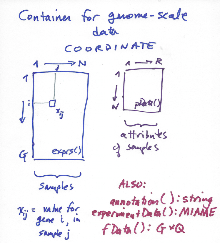
We can simplify interactions with gene expression experiments by using an object to unify the different
information sources. The following schematic helps to understand the objective. For $N$ samples, a $G \times N$
table records gene expression values. An $N \times R$ table records the sample information. The ExpressionSet object X is
designed so that X[i, j] manages genes enumerated with i and samples enumerated with j.
The ExpressionSet class is routinely used for microarray studies. To begin, we will enhance the annotation of the metadata components
rownames(sampleInfo) = sampleInfo$filename
rownames(geneAnnotation) = geneAnnotation$PROBEID
Now we build up the unified instance
library(Biobase)  # provides the class definition
es5859 = ExpressionSet(assayData=geneExpression)  # start the unification
pData(es5859) = sampleInfo  # add sample-level data
fData(es5859) = geneAnnotation  # add gene level data
es5859  # get a report
We can now program with a single data object to develop our comparative plots. We need to know that methods exprs,
fData, and [[ behave in certain ways for instances of ExpressionSet.
twoSamplePlot = function(es, stratvar, symbol, selected=1) {
    # selected parameter needed for genes that have multiple probes
    boxplot(split(exprs(es[which(fData(es)$SYMBOL==symbol)[selected],]),
                  es[[stratvar]]),xlab=stratvar, ylab=symbol)
}
twoSamplePlot(es5859, stratvar="group", symbol="BRCA2")

Adding some metadata on publication origins
The annotate package includes a function that retrieves information about the paper associated with an experiment.
library(annotate)
mi = pmid2MIAME("17206142")
experimentData(es5859) = mi
es5859
We have now bound the textual abstract of the associated paper into the ExpressionSet.
abstract(es5859)
Working with NCBI GEO to retrieve experiments of interest
Now that we have a unified representation of collections of microarrays, we can use it to manage information retrieved from GEO. The GEOquery package makes it very easy to obtain series of microarray experiments.
There are results of tens of thousands of experiments in GEO. The GEOmetadb includes tools to acquire and query a SQLite database with extensive annotation of GEO contents. The database retrieved in October 2017 was over 6 GB in size. Thus we do not require that you use this package. If you are interested, the vignette is very thorough.
We used GEOmetadb to find the name (GSE accession number) of an experiment that studied the effects of applying a compound to cells derived from glioblastoma tumors.
N.B.: The following code takes a while to run -- maybe two minutes ...
library(GEOquery)
glioMA = getGEO("GSE78703")[[1]]

# Local mirror of file in case of connection problems
#glioMA <- getGEO(filename = "/home/ubuntu/glioma/GSE78703_series_matrix.txt.gz")
glioMA
This object responds to all the methods we've already used. For example:
head(fData(glioMA))
head(pData(glioMA))
table(glioMA$`treated with:ch1`)
Now we can use our plotting function again -- with one caveat. The fields of fData are different between
the two ExpressionSets. We can update our new one fairly easily:
fData(glioMA)$SYMBOL = fData(glioMA)$"Gene Symbol" # our function assumes existence of SYMBOL in fData
twoSamplePlot(glioMA, stratvar="treated with:ch1", symbol="ABCA1") # flawed see below

Exercise
Our plot does not fully respect the design of the glioblastoma experiment. There are normal and glioblastoma-derived cells.
library(knitr)
(kable(table(glioMA$`characteristics_ch1`, glioMA$`treated with:ch1`)))
Use twoSamplePlot to compare only the normal astrocytes with respect to expression of ABCA1.
#twoSamplePlot(glioMA[, ...], stratvar="treated with:ch1", symbol="ABCA1")
Summary
- ExpressionSets unify sample-level data with molecular assays
- exprs(), fData(), pData() and associated shortcuts extract key components
- GEOquery retrieves ExpressionSets from GEO
- GEOmetadb indexes GEO and helps you find experiments for retrieval
- SummarizedExperiment and RangedSummarizedExperiment are more modern alternatives to ExpressionSet, and have different methods